
Santander Bank is interested in improving its personal product recommendation system for its customers. The bank collects marketing information about its customers, and associates it with bank account products. Currently, customers receive recommendations, but the system will provide more recommendations to some customers while neglecting others. The goal is to create a more effective product recommendation system so that the individual needs of customers are met.
Problem Description
The Santander data set contains both training data and test data. The focus of this article will be in making sense of the training data. The training data contains 48 columns: 24 are marketing data related, and the other 24 represent the products customers currently own. The marketing data will be treated as the predictor variables, while the product data will be treated as the target variables. As a forewarning to the reader, all of the column headers are in Spanish.
Marketing Data
The marketing data contains mixed (numerical and categorical) data. The only two columns that provide numerical data are renta and age. The data could possibly contain naturally occurring market segments. Perhaps a clustering algorithm could be used to find the segments. The draw back is that a valid distance metric needs to be used for the mixed data types. The following table describes the marketing data columns.
| Column names | |||
| Fecha_dato
The month from which the data originates |
Fecha_alta
Date in which customers became as the first holder of a contract in the bank |
Tiprel_1mes
Customer relation type at beginning of month A(active), I (inactive), P (former customer), R(potential) |
Tipodom
Address type. 1, primary address |
| Ncodpers
Customer code |
Ind_nuevo
New customer flag. 1 if the customer registered in the last 6 months |
Indresi
Residence index (S (yes) or N (no) if the residence country is the same as the bank’s) |
Cod_prov
Province code (customer’s address) |
| Ind_empleado
Employee index A active, B ex employed, F filial, N not employee, P pasive |
Antiguedad
Customer seniority (in months) |
Indext
Foreigner index Customer’s birth country same as bank country? (S (yes), N (no)) |
Nomprov
Province name |
| Pais_residencia
Customer’s country of residence |
Indrel
1(first/primary), 99(primary customer during the month but not at the end of the month) |
Conyuemp
Spouse index: 1 if the customer is the spouse of an employee |
Ind_actividad_cliente
Activity index (1, active customer; 0, inactive customer) |
| Sexo
Gender |
Ult_fec_cli_1t
Last date as primary customer (if he isn’t at the end of the month) |
Canal_entrada
Channel used by customer to join bank |
Renta
Gross income of household |
| Age | Indrel_1mes
Customer type at beginning of month (1 (first/pimary customer), 2(co owner), P(potential), 3(former primary), 4 (former co owner) |
Indfall
Deceased index |
Segmento
Segmentation: 01 – VIP, 02 – individuals, 03 – college graduated |
Product Data
The product data for each customer is represented using a feature vector. A one indicates if a customer has the product, and a zero indicates if the customer does not. Market basket analysis could be used to find association rules between one account and another. The association rules could then help the bank with cross-selling their products. Further, the association rules could be mined for each individual customer segment discovered from the clustering algorithm. The following table translates from Spanish to English the product columns.
| Ind_ahor_fin_ult1
Savings account |
Ind_ctma_fin_ult1
Particular account |
Ind_ecue_fin_ult1
e-account |
Ind_tjcr_fin_ult1
Credit card |
| Ind_aval_fin_ult1
Guarantees |
Ind_ctop_fin_ult1
Particular account |
Ind_fond_fin_ult1
Funds |
Ind_valo_fin_ult1
Securities |
| Ind_cco_fin_ult1
Current accounts |
Ind_ctpp_fin_ult1
Particular plus account |
Ind_hip_fin_ult1
Mortgage |
Ind_viv_fin_ult1
Home account |
| Ind_cder_fin_ult1
Derivative account |
Ind_deco_fin_ult1
Short-term deposits |
Ind_plan_fin_ult1
Pensions |
Ind_nomina_ult1
Payroll |
| Ind_cno_fin_ult1
Payroll account |
Ind_deme_fin_ult1
Medium-term deposits |
Ind_pres_fin_ult1
Loans |
Ind_nom_pens_ult1
Pensions |
| Ind_ctju_fin_ult1
Junior account |
Ind_dela_fin_ult1
Long-term deposits |
Ind_reca_fin_ult1
Taxes |
Ind_recibo_ult1
Direct debit |
Strategy
The strategy for the Santander product recommendation data set is to use clustering to discover customer segments, then to use the apriori algorithm to find bank account correlation rules for each customer segment. Since clustering algorithms rely on some notion of distance, a valid metric must be used for the mixed data types. Typically, the Euclidean distance between data points are calculated to enable clustering algorithms to work properly; however, since this data set contains categorical data, Euclidean distances will not work. Instead, the Gower distance (link to it) will be computed between data points.
The k-medoids clustering algorithm will be used instead of the k-means algorithm. This is because the centroids from the k-means clustering algorithm are sensitive to outliers, and can take on values not within the data set. K-medoids addresses these issues since it uses median values. K-modes and k-prototype were considered, but the algorithms were not readily available or implementable in Python and R. Since the number of customer segments is not known, the silhouette method will be used to discover the optimal number of clusters.
Analysis
Analysis for the Santander data set will be performed in Python and R. In addition to the analysis for the Santander data set, this article will explore the strengths and weaknesses of both languages in terms of implementation and ease. Further, this article will incorporate an aspect of super computing into the data analytics workflow.
Preprocessing The Data
The Santander analysis begins by loading in the data, and splitting the target and predictor data into variables. The Dataset class loads in the data and has subset functions to partition the data.
The data is then cleaned using functions in the CleanData class. Since the column data types are specified incorrectly, each column is formatted according to their observed data type. In addition, some of the values in the columns are not consistent. For example, indrel_1mes contains the value, “p”, but all of the other values are numerical ranging from 1 to 4. Because of this, the “p” values in the column are converted to the number 5. The data is then subdivided into months using the 17 unique values in the fecha_dato column. CSV files are written with corresponding data. The data is now ready to be processed.
|
1 2 3 4 5 6 7 8 9 10 11 12 13 14 15 16 17 18 19 20 21 22 23 24 25 26 27 28 29 30 31 32 33 34 35 36 37 38 39 40 41 42 43 |
import os import sys import csv import numpy as np import pandas as pd class SantanderAnalysis(object): def __init__(self, filepath): self.pred_vars = pd.Series() self.clustees = pd.Series() self.clusters = [] self.train_data = Dataset() self.train_data.data = self.train_data.load_data(filepath) self.get_pred_vars(self.train_data.data, 24, 1) def fix_data(self, data, column, old_dtype, new_dtype): #5, 8, 11, 15 have mixed types #age, antiguedad, indrel_1mes, conyuemp CleanData.format_col_dtype(CleanData, self.train_data, "age", "float") CleanData.format_col_dtype(CleanData, self.train_data, "antiguedad", "float") CleanData.replace_col_value(CleanData, self.train_data, "indrel_1mes", "P", "5") CleanData.format_col_dtype(CleanData, self.train_data, "indrel_1mes", "float") CleanData.format_col_dtype(CleanData, self.train_data, "conyuemp", "float") def separate_by_months(data): Dataset.write_split_data(Dataset, data, "fecha_dato") def subset_month_data(data, directory): # C:\\Users\Owner\Desktop\MGMT552\Santander\Months os.chdir(directory) sample = Dataset(data) sample_set = sample.sample_data(0.01) Dataset.write_split_data(Dataset, sample_set, "fecha_dato") def get_pred_vars(self, data, total_cols, clustee_col): print("Getting predictor data...") pred_cols = list(range(total_cols)) #predictor variable columns pred_cols.remove(clustee_col) # remove data ids self.pred_vars = data[pred_cols].copy() clustee = [clustee_col] #pandas copy function requires list self.clustees = data[clustee].values.tolist( |
Originally, the plan was to use the k-prototypes algorithm on the data set since it is recommended for mixed data; however, a readily available solution in Python capable of mining this data set was not available. Instead, the data mining was performed in R.
Data Mining in R
Luckily, an R library exists that provides an alternative solution to k-prototypes. The solution involved computing a custom distance matrix using Gower distances. The Gower distance is a metric perfectly suited for mixed data sets. Once the Gower distance matrix was computed, the PAM algorithm was used to compute the clusters.
Load Libraries
|
1 2 3 4 5 |
set.seed(1680) # for reproducibility library(dplyr) # for data cleaning library(cluster) # for gower similarity and pam library(Rtsne) # for t-SNE plot library(ggplot2) # for visualization |
Loading Data
|
1 2 3 4 5 6 |
library(readr) data_dir <- "C:/Users/Owner/Desktop/MGMT552/Santander/renta_samples/2015-12-28.csv" train_2 <- "C:/Users/Owner/Desktop/MGMT552/Santander/train_ver2.csv" data <- read_csv(data_dir) # View columns names(data) |
Exploring the data
|
1 2 3 4 5 6 7 8 9 10 |
# View columns names(data) # View summary statistics for each column summary(data) # View unique values apply(data, 2, function(x)length(unique(x))) # View column data type sapply(data, typeof) # View total number of NaNs sum(apply(data, 2, is.na)) |
The loaded data needed to be reformatted in order to compute the Gower distances. The Santander data set contains two columns that have 99% NaN values. Those columns were dropped. Further, the only columns that should be numerical are age and renta. All of the other columns were factored.
|
1 2 3 4 5 6 7 8 |
#ult_fec_cli_1t (11), conyuemp (16) clean_data <- data[c(-11,-16)] factor_data <- clean_data cols <- 1:length(clean_data) cols <- cols[! cols %in% c(6, 21)] # exclude age and renta indices factor_data[cols] <- lapply(factor_data[cols], factor) sapply(factor_data, nlevels) # how many levels does each factored column have? #sapply(factor_data, typeof) |
The predictor and target variables are separated.
|
1 2 3 4 |
pred_var <- factor_data[1:22] target_var <- factor_data[23:46] # Merge feature vector rows in target_var target_var_merge <- apply(target_var, 1, paste, collapse="") |
The PAM algorithm was run with clusters ranging from 2 – 112. The value 112 was determined by looking at the number of unique row entries in the target variable data set. This lead to the conclusion that there were 112 different classes, which meant there could be up to 112 different clusters.
|
1 2 3 4 5 6 7 8 9 |
library(plyr) #counts frequency of each unique combination rows classes <- count(target_var, vars = names(target_var)) nrow(classes) # 112 rows, therefore, 112 potential classes # sorts unique rows from most frequent to least classes[with(classes, order(-freq)), ] # *** Alternatively *** classes <- count(target_var_merge) classes[with(classes, order(-freq)), ] |
Once the Gower distance matrix computation was completed, the most similar and and dissimilar row entries were evaluated.
|
1 2 3 4 5 6 7 8 9 10 11 12 13 14 15 |
library(cluster) # for gower similarity and pam gower_dist <- daisy(pred_var[, -2], metric = "gower", type = list(logratio = 3)) summary(gower_dist) # View most similar and disimilar items gower_mat <- as.matrix(gower_dist) # Most similar pred_var[ which(gower_mat == min(gower_mat[gower_mat != min(gower_mat)]), arr.ind = TRUE)[1, ], ] # Most dissimilar pred_var[ which(gower_mat == max(gower_mat[gower_mat != max(gower_mat)]), arr.ind = TRUE)[1, ], ] |
The Gower distance matrix is evaluated using the PAM algorithm. Since there were 112 unique classes, the PAM algorithm is computed with the number of centroids ranging from 2 to 112.
|
1 2 3 4 5 6 7 8 9 10 11 12 13 14 15 |
# K-Medoids Run PAM on gower distances of marketing data ```{r} #Determine how to parallelize this for larger dataset sil_width <- c(NA) for(i in 2:112){ print(i) # print the cluster number being computed. pam_fit <- pam(gower_dist, diss = TRUE, k = i) sil_width[i] <- pam_fit$silinfo$avg.width } ``` |
The cluster number was then evaluated using the silhouette method.
|
1 2 3 4 5 6 7 8 9 10 11 12 13 14 |
Plot silhouette ```{r} # Plot sihouette width (higher is better) plot(1:112, sil_width, xlab = "Number of clusters", ylab = "Silhouette Width") lines(1:112, sil_width) ``` Using silhouette widths, the optimal number of clusters is three. However, since there are so very many more classes, it may make more sense to use a higher number of clusters in order have higher resolution in predicting which accounts customers are likely to want. The top five cluster numbers are: 3, 2, 102, 104, 103 ```{r} cluster_df <- data.frame(1:112, sil_width) # sort from highest silhouette width to least head(cluster_df[with(cluster_df, order(-sil_width)), ], 5) ``` |
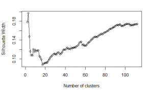
It is clear to see that the best cluster number is 3.
The cluster number assignments were then mapped to the corresponding rows in the predictor variable’s dataset. The predictor variables were then subdivided into the different clusters. At this point, the bank account product data is mapped to the respective market segments. The data is now ready to be mined for association rules using the Apriori algorithm.
|
1 2 3 4 5 6 7 8 9 10 11 12 13 14 15 16 17 18 19 20 21 22 23 24 25 26 27 28 29 30 31 32 33 34 35 36 37 38 |
pam_fit <- pam(gower_dist, diss = TRUE, k = 3) pam_results <- pred_var %>% dplyr::select(-ncodpers) %>% mutate(cluster = pam_fit$clustering) %>% group_by(cluster) %>% do(the_summary = summary(.)) pam_results$the_summary # Map clusters back to their target variables. # merged target variables with cluster numbers target_var_clusters <- data.frame(accounts = target_var_merge, cluster = pam_fit$clustering) # split target variables with cluster numbers tar_var_clusters <- data.frame(target_var, cluster = pam_fit$clustering) tar_var_clusters$cluster <- factor(tar_var_clusters$cluster) # Divide target variables into their clusters. Remove cluster number column cluster1 <- target_var_clusters[which(target_var_clusters$cluster==1), -2] cluster2 <- target_var_clusters[which(target_var_clusters$cluster==2), -2] cluster3 <- target_var_clusters[which(target_var_clusters$cluster==3), -2] # Find frequency of unique rows in each cluster. c1.classes <- count(cluster1) c1.classes <- c1.classes[with(c1.classes, order(-freq)), ] c2.classes <- count(cluster2) c2.classes <- c2.classes[with(c2.classes, order(-freq)), ] c3.classes <- count(cluster3) c3.classes <- c3.classes[with(c3.classes, order(-freq)), ] # Find differences between each cluster c1c2 <- union(cluster1, cluster2) c2c3 <- union(cluster2, cluster3) c1c3 <- union(cluster1, cluster3) c1.c2c3 <- setdiff(cluster1, c2c3) # in c1, not in c2 and c3 c2.c1c3 <- setdiff(cluster2, c1c3) # in c2, not in c1 and c3 c3.c1c2 <- setdiff(cluster3, c1c2) # in c3, not in c1 and c2 |
The unique sequences in the various clusters were compared. Cluster 1 contained the most unique sequences with 95 sequences. Cluster 2 only contained two unique sequences. Cluster 3 did not contain any unique clusters.
The three cluster centroids are defined as follows:
| Column | Cluster 1 | Cluster 2 | Cluster 3 |
| Ind_empleado | B: 1 N: 263 |
B: 1 N: 223 |
B: 0 N: 226 |
| Pais_residencia | ES: 264 | ES: 224 | ES: 226 |
| Sexo | H: 100 V: 164 |
H: 83 V: 141 |
H: 142 V: 84 |
| Age | Min: 3.00 1st Q: 38.00 Median: 45.00 Mean: 45.75 3rd Q: 53.25 Max: 90.00 |
Min: 20 1st Q: 41.75 Median: 50 Mean: 52.40 3rd Q: 63 Max: 97 |
Min: 17 1st Q: 22 Median: 24 Mean: 25.51 3rd Q: 27 Max: 62 |
| Ind_nuevo | 0: 255 1: 9 |
0: 223 1: 1 |
0: 201 1: 25 |
| Indrel | 1: 263 99: 1 |
1: 223 99: 1 |
1: 226 99: 0 |
| Indrel_1mes | 1: 264 | 1: 224 | 1: 226 |
| Tiprel_1mes | A: 254 I: 10 |
A: 10 I: 214 |
A: 38 I: 188 |
| Indresi | S: 264 | S: 224 | S: 226 |
| indext | N: 252 S: 12 |
N: 213 S: 11 |
N: 216 S: 10 |
| canal_entrada | KAT: 99 KFC: 83 KFA: 53 KHE: 14 KHK: 8 KHQ: 5 |
KAT: 92 KFC: 70 KFA: 7 KHE: 6 KCI: 5 KBZ: 4 |
KHE: 175 KHQ: 24 KFC: 12 KHD: 7 KHK: 3 |
| indfall | N: 263 S: 1 |
N: 222 S: 2 |
N: 226 S: 0 |
| Tipodom | 1: 264 | 1: 224 | 1: 226 |
| Nomprov | MADRID: 126 BARCELONA: 27 MALAGA: 14 SEVILLA: 10 VALENCIA: 9 |
MADRID: 77 BARCELONA: 27 VALENCIA: 13 ZARAGOZA: 9 CADIZ: 8 |
MADRID: 43 BARCELONA: 25 SEVILLA: 19 VALENCIA: 13 MALAGA: 12 |
| Ind_actividad_cliente | 0: 8 1: 256 |
0: 218 1: 6 |
0: 190 1: 36 |
| Renta | Min: 22416 1st Q: 75128 Median: 113960 Mean: 130795 3rd Q: 155679 Max : 784578 |
Min: 12994 1st Q: 69037 Median: 106792 Mean: 133758 3rd Q: 166061 Max: 749963 |
Min: 17493 1st Qu.: 60879 Median: 89193 Mean: 112073 3rd Qu.: 133473 Max: 791313 |
| Segmento | TOP: 23 PARTICULARES: 214 UNIVERSITARIO: 27 |
TOP: 0 PARTICULARES: 223 UNIVERSITARIO: 1 |
TOP: 0 PARTICULARES: 19 UNIVERSITARIO: 204 |
Cluster 1 is characterized by individual, middle-aged, male customers with active bank accounts that have a household income ranging from €75128 to €155679. Cluster 2 is characterized by individual, middle-aged, male customers with inactive bank accounts that have a household income ranging from €69037 to €166061. Cluster 3 is characterized by young, college-educated female adults with inactive bank accounts that have a household income ranging from €60879 to €133473.
The goal for the Apriori algorithm is to find association rules among data sets in each market segment. These association rules will then help Santander Bank make product recommendations to its customers within each respective segment.
|
1 2 3 |
library(arules) rules = apriori(target_trans, parameter=list(minlen=24, maxlen=24, support=0.01, confidence=0.5)) inspect(head(sort(target_trans, by="lift"),10)) |
Since we are only concerned with active customers, we will only evaluate rules from cluster 1. The Apriori algorithm identified two association rules with a lift greater than 2 and confidence greater than 80%. The association rules are as follows:
- A customer will likely bundle a payroll account with a pensions account
- A customer will likely bundle a direct debit account with a current account